Elongation of a model neurite over time in three growth modes (McLean and Graham, 2004; Graham et al., 2006). Achieved steady-state lengths are stable in each case, but there is a prominent overshoot and retraction before reaching steady state in the moderate growth mode.
Figure Code examples.all
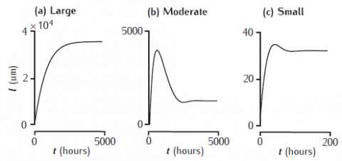
Elongation of a model neurite
Simulation environment:
Notes
Unzip the file and run CMNG_main.m in Matlab. It takes a little while to run the simulations before plotting the results.
Download:
Simulation of the Dual Constraint Model
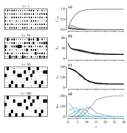
The Dual Constraint model applied to the mouse lumbrical muscle. Left hand column shows the development through time of the pattern of connectivity as displayed in a connection matrix Cnm. The area of each square indicates the strength of that element of Cnm. For clarity, only twenty of the 240 endplates are shown. Right hand column shows the development through time of four different quantities. (a) The value of Cn1, i.e. the strength of connections from each of the six axons competing for the first muscle fibre (Equation 10.13). (b) The value of the amount of available presynaptic resource An at each of the six axons (Figure 10.14). (c) The motor unit size νn of each of the six axons. (d) The number of endplates μ which are singly, or multiply innervated. The colour of the line indicates the level of multiple innervation, ranging from 1 (black) to 6 (blue). Parameters: N = 6, M = 240, A0 = 80, B0 = 1, α = 45, β = 0.4, γ = 3, δ = 2. Only terminals larger than θ = 0.01 were considered as being viable. Terminals that were smaller than this value were regarded as not contributing to νn and therefore did not receive a supply of A.
Simulation environment:
Download:
Membrane potential in a cable
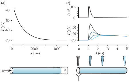
(a) Steady state membrane potential as a function of distance in a semi-infinite cable in response to current injection at one end (x = 0 µm). The parameters are d = 1µm, Ra = 35.4 Ωcm, Rm = 10kΩcm2, which, from Equation 2.26, gives the length constant λ = 840 µm. (b) Top: a simulated excitatory postsynaptic current (EPSC). Below: the membrane potential measured at different points along a cable in response to the EPSC evoked at the left-hand end of the cable. The colour of each trace corresponds to the locations of the electrodes. The neurite is 500 µm long and other parameters are the same as the semi-infinite cable shown in (a).
Simulation environment:
Notes
There are separate simulation files for (a) and (b). To run either simulation:
- In the RunControl window click on Init & Run.
- The time course of the membrane potential at various locations along the axon appears in the Graph[0] window.
- The membrane potential as a function of distance along the axon in appears in the Graph[1] window.
To observe how the spatial distribution of the membrane potential varies over time:
- In the RunControl window click on Init (mV).
- In the RunControl window click on Continue for (ms) repeatedly.
Download:
Membrane action potential
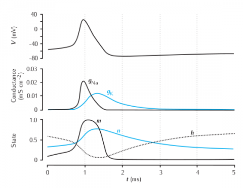
The time courses of membrane potential, conductances and gating variables during an action potential.
Simulation environment:
Download:
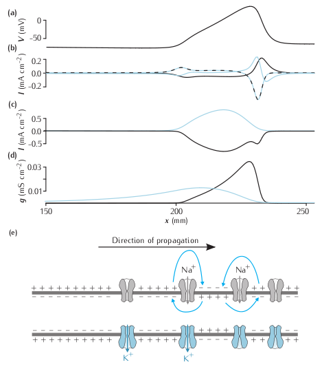
Propagating action potential
Currents flowing during a propagating action potential. (a) the voltage along an axon at one instant in time during a propagating action potential. (b) The axial current (blue line), the ionic current (dashed black-blue line) and the capacitative current (black line) at the same points. (c) The sodium (black) and potassium (blue) contributions to the ionic current. The leak current is not shown. (d) The sodium (black) and potassium (blue) currents. (e) Representation of the state of ion channels, the membrane and local circuit current along the axon during a propagating action potential.
Simulation environment:
Notes
Due to the constraints of NEURON, not all the currents in the plot from the book are displayed by NEURON as the simulation proceeds. Of the currents in (b) in the figure, only the capacitative current (i_cap in NEURON) is plotted directly by NEURON. Both the sodium and potassium currents from (c) are shown directly (ina and ik). The total ionic current in (b) is obtained by summing the sodium, potassium and leak currents (ina, ik and il_hh). The axial current is obtained using the equation I = -IC - Ii .
Download:
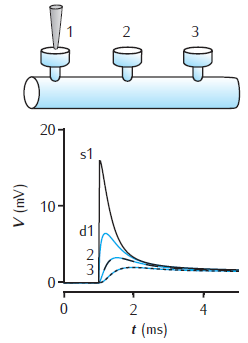
Spines on a dendrite
Voltage response to a single synaptic EPSP at a spine on a dendrite. There are three spines 100 μm apart on a 1000 μm long dendrite of 2 μm diameter. EPSP occurs at spine 1. Black lines show the voltage at each spine head. Blue lines are the voltage response in the dendrite at the base of each spine. Dendrite modelled with 1006 compartments (1000 for main dendrite plus 2 for each spine); passive membrane throughout with Rm = 28 kΩ cm2, Ra = 150 Ω cm, Cm = 1 μF cm−2; spine head: diameter 0.5 μm, length 0.5 μm; spine neck: diameter 0.2 μm, length 0.5 μm. For a similar circuit see Woolf et al. (1991).
Simulation environment:
Download:
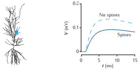
Effect of spines on somatic voltage response
Somatic voltage response to a single synaptic EPSP on a spine at a distance of 500 μm in the apical dendrites of a CA1 pyramidal cell model (blue dot on cell image). The voltage amplitude is reduced (black line) when 20,000 inactive spines are evenly distributed in the dendrites, compared to when no spines are included (blue dashed line). The somatic voltage response is corrected if Rm is decreased and Cm is increased in proportion with the additional membrane area due to spines
(blue dotted line). The CA1 pyramidal cell is n5038804, as used in Migliore et al. (2005); model has 455 compartments (with no spines); passive membrane throughout with Rm = 28 kΩ cm2, Ra = 150 Ω cm, Cm = 1 μF cm−2; spine head: diameter 0.5 μm, length 0.5 μm; spine neck: diameter 0.2 μm, length 0.5 μm; 20,000 spines increase the total membrane area by 1.4 and reduce the somatic voltage response by around 30%. For a similar comparison see Holmes and Rall (1992b).
Simulation environment:
Notes
Simulation starts with no spines. Use the "Control" panel (which may initially be hidden behind other windows) to add and delete spines, or to adjust membrane resistance and capacitance to compensate for spines. Note that adding spines may take several minutes and the subsequent simulation runs more slowly.
Download:
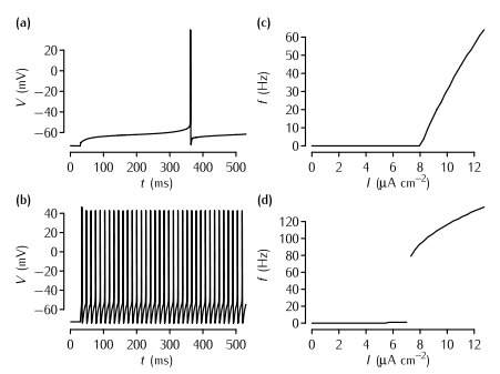
Simulation of the effect of A-type current on neuronal firing
The effect of the A-type current on neuronal firing in simulations. (a) The time course of the membrane potential in the model described in Box 5.2 in response to current injection of 8.21 µA cm2 that is just superthreshold. The delay from the start of the current injection to the neuron firing is over 300 ms. (b) The response of the model to a just suprathreshold input (7.83 µA cm2) when the A-type current is removed. The spiking rate is much faster. In order to maintain a resting potential similar to the neuron with the A-type current, the leak equilibrium potential EL is set to -72.8 mV in this simulation. (c) A plot of firing rate f versus input current I in the model with the A-type conductance shown in (a). Note the gradual increase of the firing rate just above the threshold, the defining characteristic of Type I neurons. (d) The f-I plot of the neuron with no A-type conductance shown in (b). Note the abrupt increase in firing rate, the defining characteristic of Type II neurons.
Simulation environment:
Notes
Once the simulation file is open, these are the steps to reproduce each figure:
Panel (a)
- In the top Parameters window, click on the checkbox next to Type I parameters
- Click on Set Type I threshold current
- Click on Init & Run in the Run Control window
Panel (b)
- In the top Parameters window, click on the checkbox next to Type II parameters
- Click on Set Type II threshold current
- Click on Init & Run in the Run Control window
Panel (c)
- In the top Parameters window, click on the checkbox next to Type I parameters
- Click on Plot in the Grapher window
- Simulations for a number of levels of current injection will be run and the firing frequency will be plotted against current in the Grapher window.
- Once the simulations have run, to make sure you can see these results, right-click in this graph area and select View... -> View = Plot
Panel (d)
As for panel (c), except in step 1, click on the checkbox next to Type II parameters.
Download:
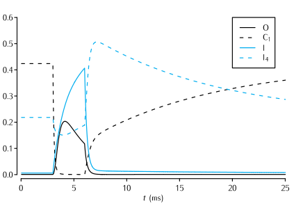
The Vandenberg and Bezanilla (1991) model of the sodium channel
Time evolution of a selection of the state variables in the Vandenberg and Bezanilla (1991) model of the sodium channel in response to a 3 ms long voltage pulse from -65 mV to -20 mV, and back to -65 mV. See Scheme 5.7 for the significance of the state variables shown. In the interests of clarity, only the evolution of the state variables I, O, I4 and C1 are shown.
Simulation environment:
Notes
To reproduce the simulation:
- In the I/V Electrode window click on the VClamp checkbox
- In the Run Control window click on Init & Run
To view the channel's kinetic scheme, in the ChannelBuild[0] window click on highlighted text O: 9 state, 9 transitions.
Download:
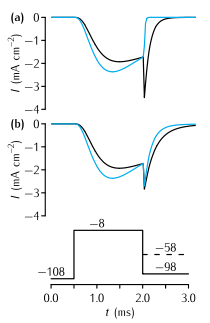
Tail currents in the Vandenberg and Bezanilla (1991) model and the Hodgkin and Huxley (1952d) model
Tail currents in the Vandenberg and Bezanilla (1991) model (VB, black traces) and the Hodgkin and Huxley (1952d) model (HH, blue traces) of the sodium current in squid giant axon in response to the voltage-clamp protocol shown at the base, where the final testing potential could be (a) -98mV or (b) -58mV. During the testing potential, the tail currents show a noticeably slower rate of decay in the VB model than in the HH model. To assist comparison, the conductance in the VB model was scaled so as to make the current just before the tail current the same as in the HH model. Also, a quasi-ohmic I-V characteristic with the same ENa as the HH model was used rather than the GHK I-V characteristic used in the VB model. This does not affect the time constants of the currents, since the voltage during each step is constant.
Simulation environment:
Notes
This simulation contains two separate neurons, one containing VB model sodium channels and one containing HH model sodium channels. The parameters of each neuron are described in the windows entitled somavb and somahh. Each neuron has a voltage clamp electrode inserted.
To reproduce panel (a):
- In both I/V Clamp Electrode windows click on the checkbox next to VClamp
- In the Run Control window click on Init & Run
- The currents shown in Fig 5.13a should appear in the middle graph on the right. Additionally, the upper graph shows the states of the VB channel (see Fig 5.12) and the lower graph shows the conductance of the two types of channels
To reproduce panel (b)
- In both I/V Clamp Electrode windows in the Return Level section change the amplituce to -58mV
- In the Run Control window click on Init & Run
Download:
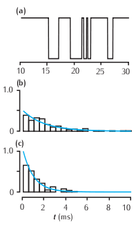
Features of a two-state kinetic scheme
Features of a two-state kinetic scheme. (a) Simulated sample of the time course of channel conductance of the kinetic scheme described in Scheme (5.13). The parameters are α = 1 ms-1 and β = 0.5 ms-1. (b) Histogram of the open times in a simulation and the theoretical prediction of 0.5e-0.5t from Equation 5.14. (c) Histogram of the simulated closed times and the theoretical prediction e-t.
Simulation environment:
Notes
To run the simulation:
- In the Run Control window click on Init & Run
- In the top graph a trace of the conductance of the channel should appear. In the middle and lower graphs histogram of the open and closed time distributions with theoretical predictions should appear.
To change the rate of the opening and closing:
- In the ChannelBuild[0] window click on O: 2 state, 1 transitions
- In the ChannelBuildGateGUI window that opens, change the values in the boxes at the lower right. The forward rate (α in the figure) is aCO and the backard rate β is aCO.
Download:
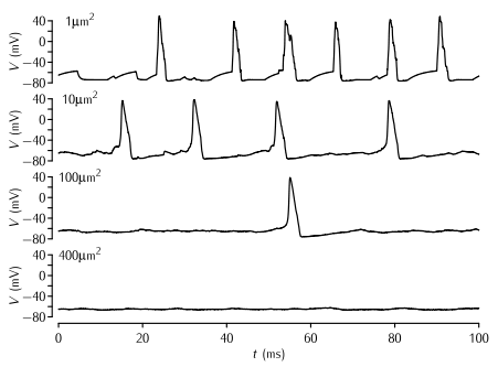
Action potentials due to stochastic sodium and potassium channels
Simulations of patches of membrane of various sizes with stochastic Na+ and K+ channels. The density of Na+ and K+ channels is 60 channels per µm2 and 18 channels per µm2 respectively, and the single channel conductance of both types of channel γ = 2 pS. The Markov kinetic scheme versions of the Hodgkin-Huxley potassium and sodium channel models were used (Schemes 5.5 and 5.8). The leak conductance and capacitance is modelled as in the standard HH model. No current is applied; the action potentials are due to the random opening of a number of channels taking the membrane potential to above threshold.
Simulation environment:
Notes
To produce a trace similar to the top trace in the figure:
- In the Run Control window click on Init & Run.
- A trace similar to the top one in the figure will appear in the top right graph. Below this is a graph of the sodium and potassium currents.
To reproduce each of the other panels from the figure:
- In the soma window change the length L of the soma to the area of membrane you wish to simulate. Since the diameter of the neuron is 1/π the neuron's area in µm2 is equal to its length in µm.
- In the PointProcessGroupManager window click on nahh[0]. In the panel on the right set Nsingle to 18 multiplied by the area in µm2. For example if the area is 10µm2, Nsingle should be 180. This step is necessary because the NEURON PointProcess describes the number of channels inserted rather than their density. To maintain a constant density, the number of channels has to be scaled in line with the area.
- In the PointProcessGroupManager window click on khh[0]. In the panel on the right set Nsingle to 60 multiplied by the area in µm2. For example if the area is 10µm2, Nsingle should be 600.
- In the Run Control window click on Init & Run. Traces should appear as above.
To investigate the kinetic schems of the sodium and potassium channels:
- In the ChannelBuild[0] window click on O: 8 state, 10 tranisitions. This shows the sodium kinetic scheme.
- In the ChannelBuild[1] window click on O: 5 state, 4 tranisitions. This shows the potassium kinetic scheme.
Download:
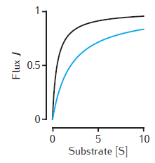
Michaelis-Menten kinetics
Two examples of the enzymatic flux, J, as a function of the substrate concentration, [S], for Michaelis-Menten kinetics (Equation 6.1). Arbitrary units are used and Vmax = 1. Black line: Km = 0.5. Blue line: Km = 2. Note that half-maximal flux occurs when [S] = Km.
Simulation environment:
Download:
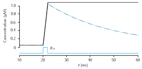
Calcium transients in a cylindrical compartment
Calcium transients in a 1.0 single cylindrical compartment, 1 μm in diameter and 1 μm in length (similar in size to a spine head). Initial concentration is 0.05 μM. Influx is due to a calcium current of 5 μA cm−2, starting at 20 ms for 2 ms, across the radial surface. Black line: accumulation of calcium with no decay or extrusion. Blue line: simple decay with τdec = 27 ms. Gray dashed line: instantaneous pump with Vpump = 4 × 10⁻⁶ μMs−1, equivalent to 10−11 mol cm−2 s−1 through the surface area of this compartment, Kpump = 10 μM, Jleak = 0.0199 × 10⁻⁶ μMs−1.
Simulation environment:
Download:
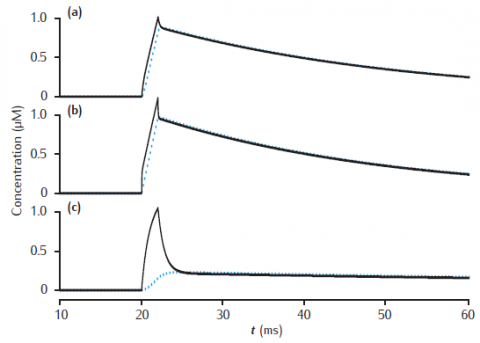
Calcium transients in a submembrane shell
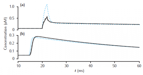
Calcium transients in the submembrane shell (black lines) and the compartment core (blue dashed lines) of a two pool model that includes a membrane-bound pump and diffusion into the core. Initial concentration Ca0 is 0.05 μM throughout. Calcium current as in Figure 6.3. Compartment length is 1 μm. (a) Compartment diameter is 1 μm, shell thickness is 0.1 μm; (b) Compartment diameter is 1 μm, shell thickness is 0.01 μm; (c) Compartment diameter is 4 μm, shell thickness is 0.1 μm. Diffusion: DCa = 2.3 × 10⁻⁶ cm2 s−1; Pump: Vpump = 10−11 mol cm−2 s−1, Kpump = 10 μM, Jleak = Vpump ∗ Ca0/(Kpump + Ca0).
Simulation environment:
Download:
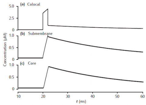
Calcium transients in a three pool model
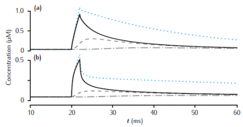
Calcium transients in (a) the potassium channel colocalised pool, (b) the larger submembrane shell, (c) the compartment core in a three pool model. Note that in (a) the concentration is plotted on a different scale. Compartment 1 μm in diameter with 0.1 μm thick submembrane shell; colocalised membrane occupies 0.001% of the total membrane surface area. Calcium influx into the colocalised pool. Calcium current, diffusion and membrane-bound pump parameters as in Figure 6.5.
Simulation environment:
Download:
Calcium transients for different numbers of shells
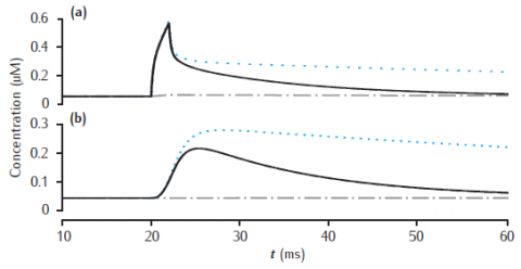
Calcium transients in the (a) submembrane shell and (b) cell core (central shell) for different total numbers of shells. Black line: 11 shells. Gray dashed line: 4 shells. Blue dotted line: 2 shells. Diameter is 4 μm and the submembrane shell is 0.1 μm thick. Other shells equally subdivide the remaining compartment radius. All other model parameters are as in Figure 6.5.
Simulation environment:
Notes
Note that the simulation plots correctly show the calcium transients all beginning after the stimulus at 20 msecs, unlike the figure in the book in which part (b) has a spurious time shift! (This is a drawing error, not a simulation error).
Download:
Longitudinal diffusion of calcium
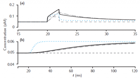
Longitudinal diffusion along a 10 μm length of dendrite. Plots show calcium transients in the 0.1 μm thick submembrane shell at different positions along the dendrite. Solid black line: 0.5 μm; dashed: 1.5 μm; dot-dashed: 4.5 μm. (a) Diameter is 1 μm. (b) Diameter is 4 μm. Calcium influx occurs in the first 1 μm length of dendrite only. Each of ten 1 μm long compartment contains four radial shells. Blue dotted line: calcium transient with only radial (and not longitudinal) diffusion in the first 1 μm long compartment. All other model parameters as in Figure 6.5.
Simulation environment:
Notes
Simulation does not reproduce calcium transient without longitudinal diffusion (blue dotted line in figure).
Download:
Calcium transients with slow buffer
Calcium transients in (a) the 0.1 μm thick submembrane shell and (b) the cell core of a single dendritic compartment of 4 μm diameter with 4 radial shells. Slow buffer with initial concentration 50 μM, forward rate k+ = 1.5 μM-1s−1 and backward rate k− = 0.3 s−1. Blue dotted line: unbuffered calcium transient. Gray dashed line (hidden by solid line): excess (EBA) approximation. Gray dash-dotted line: rapid (RBA) buffer approximation. Binding ratio κ = 250. All other model parameters as in Figure 6.5.
Simulation environment:
Notes
Use Parameters panel in GUI to change parameter values for buffered model, EBA and RBA simultaneously. Same code can generate results for both figures 6.12 and 6.13.
Download:
Calcium transients with fast buffer
Calcium transients in (a) the 0.1 μm thick submembrane shell and (b) the cell core of a single dendritic compartment of 4 μm diameter with 4 radial shells. Fast buffer with initial concentration 50 μM, forward rate k+ = 500 μM-1s−1 and backward rate k− = 1000 s−1. Black solid line: fixed buffer. Blue dotted line: mobile buffer with diffusion rate Dbuf = 1 × 10⁻⁶ cm2 s−1. Gray dashed line: excess (EBA) approximation. Gray dash-dotted line: rapid (RBA) buffer approximation. Binding ratio κ = 25. All other model parameters as in Figure 6.5.
Simulation environment:
Notes
Use Parameters panel to change all parameter values. Code produces results for figures 6.12 and 6.13.
Download: